Temperature Field of a Two Cylinders with a Thermal Resistance Between them

Let us consider a problem of distribution of temperature field of a system of two embedded cylindrical bodies with a thermal resistance on the contact surface. The radius of internal body is equal to r2=50 mm, and the radius of external body is equal to r1=70 mm. Both cylinders are located on the same level and have the height equal to D=70 mm. Zero heat flux is prescribed on the circular surfaces of these bodies. On the lateral surface of the external cylinder there is a heat exchange with an ambient environment with the heat transfer coefficient equal to H=120 W/(m2 • oK) and the temperature of the ambient environment equal to  T0=293.15 oK. Along the central segment of the cylinder along the entire height we prescribe the heat power P=200 W. On the interface between two cylinders we prescribe the thermal resistance of magnitude R=0.01 oK•m2/W. The thermal conductivity of the internal cylinder is equal to K2=50 W/(m • oK), and external cylinder К1=50 W/(m • oK) [Alloy Steel (SS)].

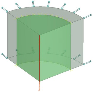
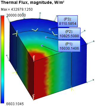
We consider only one quarter of the entire cylindrical system of bodies. The symmetry condition can be satisfied by assuming zero heat flux on the rectangular boundaries of the structure. The power on the central segment must then be divided by four (distributed between two bodies). P1/4=P/4=50 W. An example of such construction is shown below. (see figure).

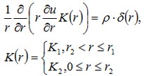
The differential equation for a point source has the form:

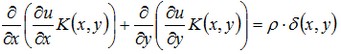
where ρ – density of distributed power. For our case: ρ = P / D. K – is a function of thermal conductivity of the material of the cylinders. K(x,y)=K1 if a point (x,y) belongs to the external cylinder, K(x,y)=K2 if a point belongs to the internal cylinder, δ – is a function of the heat source (Dirac function). Solution of this differential equation is a Green’s function G (heat source function). Equation is represented in the coordinates (x,y). But the solution will actually depend only on one variable – radial coordinate (distance from the segment with the applied power), and will have the form:

The boundary condition for this problem corresponds to the heat transfer by convection

Solution for this problem has the form:

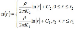
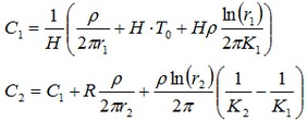
where the constants C1 and C2 are determined from the condition of the temperature jump on the interface between two bodies and the boundary condition. Expressions that determine C1 and C2 have the form:

Condition of the temperature jump has the form:

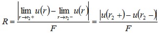
where F – thermal heat flux on the boundary can be found by the formula:

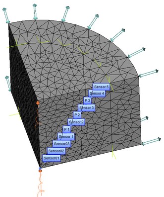
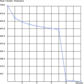
Let us locate the sensors of the temperature as shown on the Figure and make a plot for them at x=y=20,30,40 mm, that correspond to radii r =|x|√2=28.28427; 42.42640; 56.56854 mm. In the given points we will compare the numerical solution obtained using AutoFEM Analysis with the analytical solution.

After carrying out calculation the following results are obtained:

Table 1. Parameters of finite element mesh

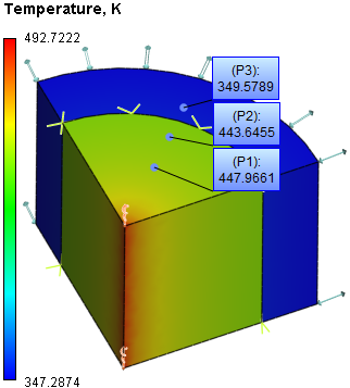
Table 2. Result "Temperature"

 

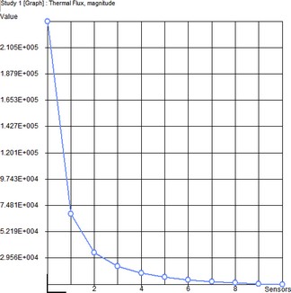
In addition, let us check the magnitude of the heat flux. Notice that unlike the temperature, the heat flux does not have a jump on the interface between the materials, i.e., is a continuous function of space. It can be evaluated as:

Table 3. Result "Thermal flux, W/m2"

Conclusions:

The relative error of the numerical solution compared with the analytical solution not exceed 1.7% for linear elements.

We confirmed the continuity of the thermal heat flux, physically important for the thermal systems.

At the neighborhood of the concentrated source (point or segment) of the heat power, the errors of the linear and quadratic elements do not differ significantly. This is related to the fact that the temperature for such heat sources is unbounded. At a certain distance from them, the quadratic elements show superior accuracy compared to the linear elements.

Although the unbounded value of the temperature cannot represent a real physical model, it allows us to examine different heat sources, for example, thin wires or objects sufficiently remote from the domain of interest.

*The results of numerical tests depend on the finite element mesh and may differ slightly from those given in the table.

 

Read more about AutoFEM Thermal Analysis

autofem.com

Return to contents