Orthotropic Graphite Plate under Steady State Temperature Regime

Let us consider now the problem of steady state temperature field distribution for a plate with orthotropic thermal conductivities of a crystalline material one of the edges of which is held at a constant temperature Т1, and the remaining edges are at Т2.

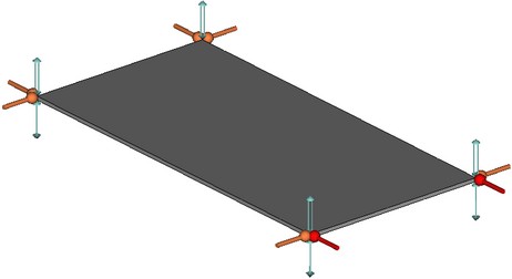
As an example, let us consider a rectangular graphite plate with the thermal conductivity of K1=278 W/(m • oK) along the principle direction and K2=139 W/(m • oK) in a perpendicular direction. The dimensions are: 200 mm х 100 mm. Parameters are a=200 mm, b=100 mm. The plate is elongated along the principle direction. Let us apply the temperature of T=353.15 oK to one of the edges of smaller size. In the steady-state regime the temperature is constant and does not depend on time. The temperature of 273.15 oK is applied to the remaining of the edges. Over the entire surface (from both sides) a heat exchange with the ambient environment takes place. The temperature of the ambient environment is 273.15 oK, the heat transfer coefficient is H=400 W/(m2 • oK). The thickness of the plate is D=2 mm. (see figure).

For the given problem, the differential equation has the form:

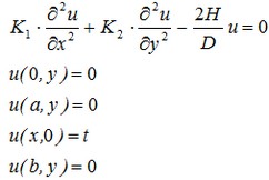
This problem can be solved in the OXY-coordinate plane, on a rectangular domain [0,a]х[0,b], associated with the graphite plate.

Analytical solution of the problem is expressed in terms of Fourier series and has the form :

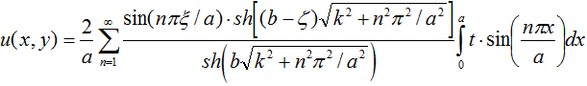
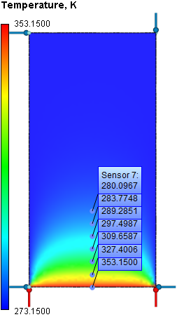
The isothermal lines of the obtained solution have the form shown on the Figure (obtained with Maple 9.5):

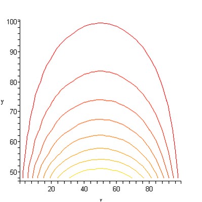
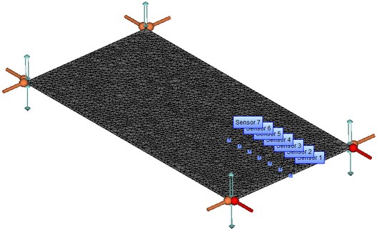
Let us locate the sensors of the temperature as shown on the Figure and make a plot for them at x=50 mm, y=10,20,30,…60 mm. In the given points we will compare the numerical solution obtained using AutoFEM Analysis with the analytical solution.

The finite element model with applied boundary conditions

Let us compare analytical solution with the solution obtained from AutoFEM. Notice that the points that are closer to the boundary do not have to be selected (200 terms in a sum is acceptable for 8-10 mm), since Fourier series will converge at these points with large oscillations. To obtain better accuracy, it is necessary to increase the number of terms in a partial sum of a series. After carrying out calculation the following results are obtained:

Table 1. Parameters of finite element mesh

Finite element type	Number of nodes	Number of finite elements
linear tetrahedron	5134	15910

Table 2. Result "Temperature"

Distance from the center, mm	Numerical solution Temperature T*, K	Analytical solution Temperature T, К	Error δ = 100%* \|T* - T\| / \|T\|
10	327.4006	327.3429	0.02
20	309.6587	309.6093	0.02
30	297.4987	297.4952	0.002
40	289.2851	289.2882	0.001

Conclusions:

The relative error of the numerical solution compared with the analytical solution not exceed 0.02% for linear elements.

The present method was proven to be effective when solving the problems with anisotropic distribution of temperatures. The existence of orthotropic properties did not affect the computational efficiency of the method.

The plot of dependence of the temperature on distance shows that the analytical and numerical solutions coincided from a practical point of view. This implies that distributions of temperature maximums and minimums are identical, and hence, the calculation of heat flux and power will be carried out with the same degree of accuracy.

*The results of numerical tests depend on the finite element mesh and may differ slightly from those given in the table.

autofem.com

Return to contents