Isotropic Plate under Heat Flux and Convection

Isotropic Plate under Heat flux and Convection

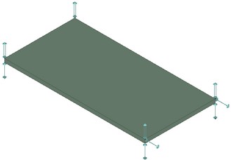
Let us consider a steel plate b x a=100x200 mm of thickness D=5 mm with the thermal conductivity of K=50 W/(m oK) [Alloy Steel (SS)]. Let us show that the steady-state heat transfer problem can also be solved for the case when on the boundary the temperature is not held constant (for correct modeling the temperature must be known in advance). Let us consider two types of loads: heat flux (equal to zero for some boundaries) and heat transfer by convection. On the surface of the plate (from both sides) we prescribe the heat exchange with ambient environment with the heat transfer coefficient C=40 W/(m2 • oK) and the temperature of the ambient environment equal to zero. On the fourth side (of length 100 mm) we prescribe a convective heat transfer with the coefficient H=20 W/(m2 • oK) and the temperature of the ambient environment equal to u0=283.15 oK. (see figure).

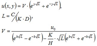
Let us locate the origin of the coordinate system at the corner of the plate, let the OY-axis be directed along the longer side of the plate, and convection will then be applied to the edge y=b. Then we will infer that two out of three edges, on which a zero heat flux is prescribed, correspond to the values x=0 and x=a. This means that the solution that we obtain must not depend on the coordinate x. Solution will have the form:

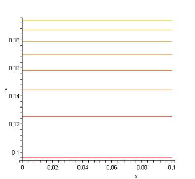
Below we show the isothermal lines for the solution obtained using the Maple software.

Convection is applied for the coordinate Y=b.

Isothermal lines for the solution obtained using the Maple software. Convection is applied to the edge y=b. When y=0 the thermal heat flux is zero

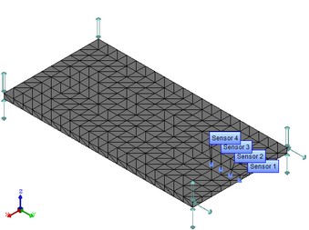
Let us locate the sensors of the temperature as shown on the Figure and make a plot for them at y=170; 180; 190; 200 mm. In the given points we will compare the numerical solution obtained using AutoFEM Analysis with the analytical solution.

The finite element model with applied boundary conditions

After carrying out calculation the following results are obtained:

Table 1. Parameters of finite element mesh

Finite element type	Number of nodes	Number of finite elements
linear tetrahedron	462	1200

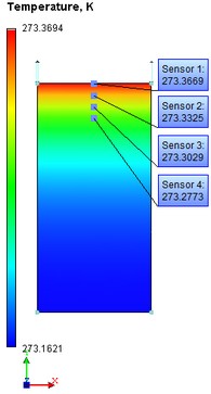
Table 2. Result "Temperature"

Coordinate y, mm	Numerical solution Temperature T*, K	Analytical solution Temperature T, К	Error δ = 100%* \|T* - T\| / \|T\|
170	273.2773	273.2783	3.55E-04
180	273.3029	273.3033	1.43E-04
190	273.3325	273.3332	2.67E-04
200	273.3669	273.3690	7.86E-04

Conclusions:

The relative error of the numerical solution compared with the analytical solution not exceed 0.0008% for linear elements.

The problem was solved almost exactly with minimum computational cost.

*The results of numerical tests depend on the finite element mesh and may differ slightly from those given in the table.

autofem.com

Return to contents