| AutoFEM Analysis Non-Stationary Temperature Field in an Orthotropic Plate | |||||||
| AutoFEM Analysis Non-Stationary Temperature Field in an Orthotropic Plate | |||||||
Non-Stationary Temperature Field in an Orthotropic Plate
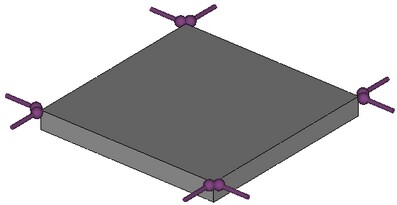
Let us compare a two-dimensional problem of cooling of a graphite plate with orthotropic properties. The initial temperature of the plate is t0=60 °С. The temperature on the boundary of the plate is maintained equal to zero. The plate cools down during the period of 20 seconds. Let us determine the temperature field at the moments of time t1-4 = 2, 5, 10 sec. Calculation of the temperature field will be conducted for control points 1-5 with coordinates (Xi,Yi):
i |
1 |
2 |
3 |
4 |
5 |
X, mm |
20 |
20 |
80 |
80 |
50 |
Y, mm |
20 |
80 |
20 |
80 |
50 |
|
The material coordinate system of the body is chosen such that the origin of the coordinate system coincides with the angle of the plate, and the base direction is selected along the OY-axis.
Properties of the orthotropic plate: density ρ=2.5 g/cm3, specific heat c=840 J/(kg •°K), coefficients of thermal conductivity: K1=0.139 W/(mm •°K) (along the OX-axis); K2=0.278 W/(mm • °K) (along the OY-axis – base direction). The plate has a rectangular shape 100 × 100 mm.
Differential equation has the form:
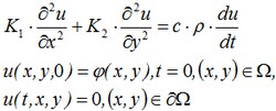
where ∂Ω – the boundary of the numerical domain. Analytical solution of the problem has the form2*:
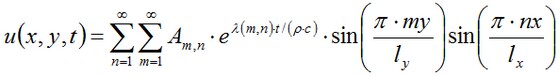
where
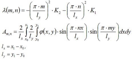
In our case x1=100, y1=100, x0=y0=0. We used n=m=60 terms in the series expansion.
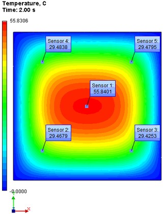
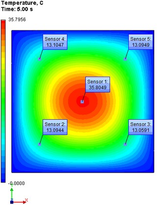
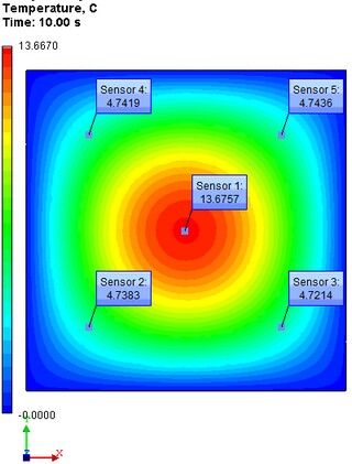
In the given points we will compare the numerical solution obtained using AutoFEM Analysis with the analytical one at the moments of time: 2, 10, 20 sec.
|
|
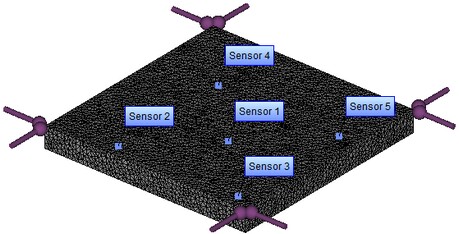
The finite element model with applied boundary conditions and sensors located at a coordinate x=20,y=20; x=20,y=80; x=80,y=20; x=80,y=80; x=50,y=50 mm |
After carrying out calculation the following results are obtained:
Table 1. Parameters of finite element mesh
Finite element type |
Number of nodes |
Number of finite elements |
linear tetrahedron |
18649 |
96109 |
Table 2. Parameters of of time discretization
Total calculation time (sec) |
Time step (sec) |
Number of time layers |
10 |
0.5 |
21 |
Table 3. Result "Temperature"
Calculation time t, s |
Numerical solution |
Analytical solution |
Error δ = 100% • |T* - T| / |T| |
Sensor 1-4: |
|||
2 |
29.4838 |
28.8050 |
2.36 |
5 |
13.1047 |
13.1503 |
0.35 |
10 |
4.7436 |
4.74820 |
0.10 |
Sensor 5: |
|||
2 |
55.8401 |
56.1856 |
0.61 |
5 |
35.8049 |
35.5560 |
0.70 |
10 |
13.6757 |
13.6788 |
0.02 |
|
Conclusions:
The relative error of the numerical solution compared to the analytical solution is smaller than 0.9 % on 20 s. For the given problem we obtained a realistic picture of the field.
As was already shown in the example with the heat flux on the surface of the sphere: for calculation over the large intervals of time it is preferable to use linear elements since because of the smaller number of nodes the error on the time layers is accumulated slower.
In our case thermal conductivities along the main axes of the plate are sufficiently high which implies that it will cool down very fast. That is the reason why the quadratic elements on sufficiently small intervals of time give more accurate results. The error of the solution for the non-stationary problems does not exceed 2.5 % for FE with linear elements and 2 % with quadratic elements.
*The results of numerical tests depend on the finite element mesh and may differ slightly from those given in the table.
** Solution was obtained by the method of separation of variables.
Read more about AutoFEM Thermal Analysis