Non-Stationary Temperature Field in an Isotropic Cylinder

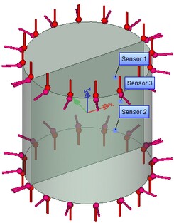
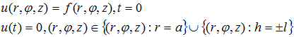
Let us consider a problem of cooling of a cylindrical body with isotropic properties that has an initial temperature of t0=60 °C inside the volume. The temperature equal to zero is maintained on the boundary of the body; cooling time does not exceed 20 sec. Let us determine the temperature in control points 1, 2, 3 that have the following coordinates in the cylindrical coordinate system (the origin of the coordinate system is located in the center of the cylinder): r1=25 mm, h1=25 mm; r2=25 mm, h2= - 25 mm; r3=30 mm, h3=0 mm at the following moments of time t1,2,3=2; 10; 20 sec.

Geometric and physical parameters of the body: height of the cylinder H =100 mm, radius of the cylinder a =50 mm. Density ρ=7700 kg/m3, specific heat c =460 J / (kg •°C), thermal conductivity K = 40 W / (m • °C). (see figure).

Let us look for the solution in the cylindrical coordinate system. The center of the coordinate system is located at the center of the cylinder in the middle cross-section (the total height - h), and the axis from which the distance is measured (radius in the cylindrical coordinate system – r) coincides with the axis of the cylinder. Denote l=H/2. Then the solution of the equation takes the form:

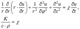
Boundary conditions for this equation have the following form:

In the boundary conditions we imply that f – some distribution of the temperature inside the body at initial moment of time, u(t)=0 on the surface of the cylindrical body during the entire period of time. We notice that in our case f – is a constant.

Let us represent the solution of the given equation in the form of a series in harmonic and Bessel functions for more general case when f is not a constant.

where χ=K/(c • ρ) is the coefficient of temperature conductivity, Jn (r) – Bessel function, parameter μ is a root of the equation Jn (a μ) =0

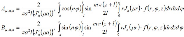
The coefficients A and B can be calculated according to the formulas shown below:

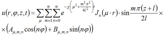
In our simple case when f = t0 from the entire series over n we have only the first term left corresponding to n=0. But expansion over m and μ must be considered. The simplified form of the solution can be written as:

where

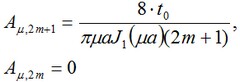
i.e., in the sum over m we retain only the odd coefficients.

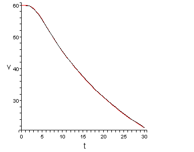
Let us compare the value of the temperature at a fixed point at different moments of time with the solution obtained by the finite element method. The point will be selected at a sufficiently large distance from the main axis of the cylinder, for better convergence of the series in the analytical solution (the equation has a singularity of the type 1/r which significantly affects the convergence of the series of Bessel functions).

In the given points we will compare the numerical solution obtained using AutoFEM Analysis with the semi-analytical one at the moments of time: 2, 10, 20 sec.

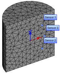
The finite element model with applied boundary conditions and sensors located at a coordinate r=25,h=25; r=25,h=-25; r=30,h=0 mm

Since the alternative solution was obtained by the semi-analytical approach (by extraction of partial sums of the series), it is required to determine the number of significant digits which can be used for comparison with analytical solution. Table given below shows with what accuracy the calculations were carried out for obtaining solution by the series expansion and for construction of the solution plot. Conclusion about the number of significant digits in the analytical solution can be made by the indicator of the relative change in the solution and the fact that our series always converges.

After carrying out calculation the following results are obtained:

Table 1. Parameters of finite element mesh

Finite element type	Number of nodes	Number of finite elements
linear tetrahedron	9200	6091

Table 2. Parameters of of time discretization

Total calculation time (sec)	Time step (sec)	Number of time layers
20	0.5	41

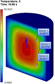
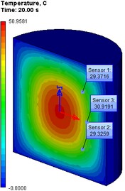
Table 3. Result "Temperature"

Calculation time t, s	Numerical solution Temperature T*, °C	Analytical solution Temperature T, °C	Error δ = 100% • \|T* - T\| / \|T\|
Sensor 1: r = 25, h = 25 mm
2	59.9324	59.9710	0.06
10	46.6873	46.7052	0.04
20	29.3716	29.5316	0.54
Sensor 2: r = 25, h = –25 mm
2	59.9853	59.9710	0.02
10	46.6211	46.7052	0.18
20	29.3259	29.5316	0.70
Sensor 3: r = 30, h = 0 mm
2	59.8067	59.7728	0.06
10	45.2759	45.5215	0.54
20	30.9191	31.1765	0.83

Conclusions:

The relative error of the numerical solution compared to the analytical solution is smaller than 0.9 % on 20 s. The calculation error is stable in time and does not grow significantly when the computational time is increased. Plot of dependence of temperature on time shows that analytical and numerical solutions practically coincided. The method turned out to be effective for solution of the problems with complex geometry.

When using quadratic elements the number of nodes is significantly larger than that for linear elements. Hence, with time (for each new time layer), quadratic elements accumulate larger error than linear elements. As can be see, in 20 seconds, i.e., for relatively small time interval for our problem, quadratic elements are more accurate than linear elements, but on the significantly larger time interval the calculation error with quadratic elements became even larger.

*The results of numerical tests depend on the finite element mesh and may differ slightly from those given in the table.

autofem.com

Return to contents