Non-Stationary Temperature Field in an Isotropic Sphere with Convection on the Surface

Let us consider the problem of determination of the temperature at any point inside the sphere in equal increments of time Δt1,2,3 = 30, 40, 60 sec if we prescribe the initial temperature Tstart = 60 °C inside the sphere, and on the boundary of the sphere we prescribe the heat transfer by convection with the heat transfer coefficient H=300 W/(m2•°C) (the sphere that had a temperature of 60 0C inside was put down to cold sea water at a temperature of zero degrees).

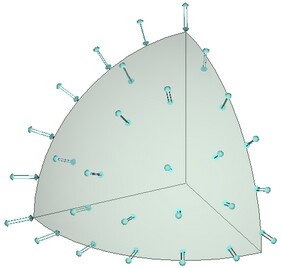
Parameters of the sphere: radius a=100 mm, density of the material 7800 kg / m3, specific heat c =440 J / (kg •°C), thermal conductivity K=50 W / (m • °C). For numerical modeling we consider a 1/8th part of the sphere. Conditions of symmetry are enforced by prescribing zero heat flux on the boundary surfaces of the sphere that have a center of the sphere as a vertex*2. (see figure).

Let v be the desired solution (temperature field). Then, by taking into account that the solution does not depend on the angles of rotation of the vector emanating from the center of the sphere (symmetry condition), we can perform the change of variables in the form v=r•u, where r – distance from the center of

the sphere, and u – some function. After this change of variables, we obtain the equation for u:

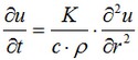
where t – is time for cooling/heating of the solid body. Boundary conditions for u:

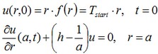
where f(r) – initial distribution of the temperature and the coefficient h = H/K. Analytical solution of this problem obtained by the method of separation of variables, is given below.

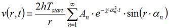
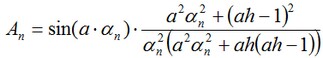
where χ=K/(c • ρ) is the coefficient of temperature conductivity. The expansion coefficients An and the values αn can be determined by the formula:

and

i.e., αn – are the roots of the last equation.

Let us compare the numerical solution with the obtained analytical solution at point with radius R1=0.5 m.

In the given point we will compare the numerical solution obtained using AutoFEM Analysis with the analytical one.

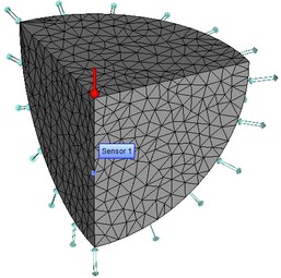
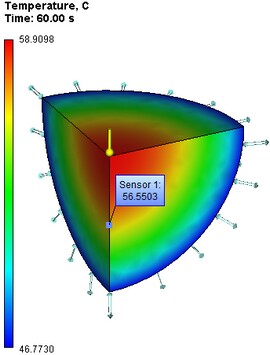
The finite element model with applied boundary conditions and a sensor located at a coordinate r=50 mm

After carrying out calculation the following results are obtained:

Table 1. Parameters of finite element mesh

Finite element type	Number of nodes	Number of finite elements
linear tetrahedron	1398	6152

Table 2. Parameters of of time discretization

Total calculation time (sec)	Time step (sec)	Number of time layers
60	1	61

Table 3. Result "Temperature"

Calculation time t, s	Numerical solution Temperature T*, °C	Analytical solution Temperature T, °C	Error δ = 100%* \|T* - T\| / \|T\|
30	59.2657	59.2381	0.05
40	58.4883	58.4375	0.09
60	56.5503	56.4123	0.24

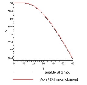
Conclusions:

We confirmed the numerical efficiency of the method. The relative error of the numerical solution compared to the analytical solution is smaller than 0.25%, which guarantees two significant digits accuracy for relatively small computational expenses of memory and time. Plot of dependence of temperature on time shows that analytical and numerical solutions practically coincided.

The calculation error is significantly smaller for quadratic elements than for linear elements, however, the time rate of growth of the error is somewhat larger for quadratic elements.

*The results of numerical tests depend on the finite element mesh and may differ slightly from those given in the table.

** On the boundaries, where no boundary conditions are specified, the zero heat flux condition is satisfied automatically.

autofem.com

Return to contents