Thermal Heat Flux in an Isotropic Disk

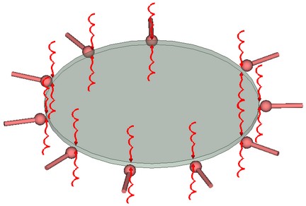
Let us consider now the problem of heating of a circular plate with the sources of heat distributed over the surface. Let us prescribe the heat flux from both sides. Around the plate along the edges we will prescribe the constant temperature.

As an example we consider a thin plate with the thermal conductivity K=75 W/(m • oK) [Ductile Iron (SN)]. The radius of the plate is R=100 mm, thickness D=5 mm. The value of the density of the heat flux is F=60 W/m2. Temperature of the edges around the plate is T=293.15 oK. (see figure).

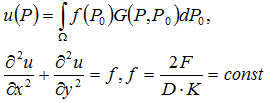
The equation that must be solved for a surface of a disk has the following form:

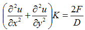
At the right side of the equation we have the volumetric density of the heat source (equivalent to a surface density for a plane problem).

Boundary conditions:

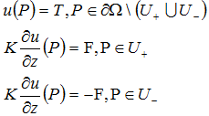
where U- and U+ - are respectively lower and upper sides of the plate. Analytical solution can be expressed in terms of the function of the heat source G(P, P0).

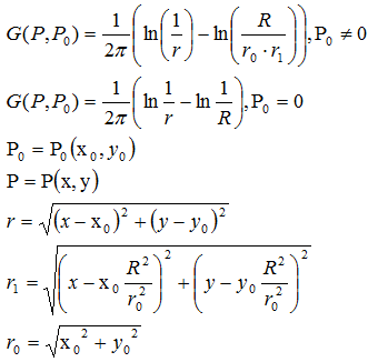
This function is a solution of the Laplace equation with the singular right-hand side (at the right side we have Dirac function) of unit power.

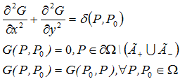
Solution of Poisson’s equation can be expressed in terms of the source function as:

Analytical solution was calculated in the Maple 9.5 system by the method of numerical integration _d01ajc (Gauss integration using 10 points and Croncord integration using 21 points). We used 6 significant digits of accuracy in the analytical solution to compare the results.

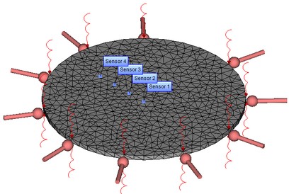
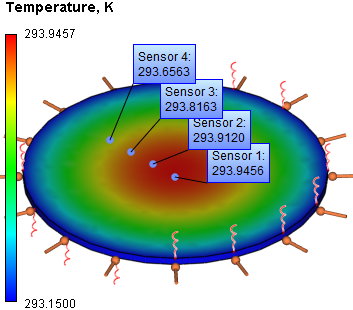
Let us locate the sensors of the temperature as shown on the Figure and make a plot for them at r =0; 20; 40; 60 mm. In the given points we will compare the numerical solution obtained using AutoFEM Analysis with the analytical solution.

The finite element model with applied boundary conditions

After carrying out calculation the following results are obtained:

Table 1. Parameters of finite element mesh

Finite element type	Number of nodes	Number of finite elements
linear tetrahedron	462	1200

Table 2. Result "Temperature"

Radius r, mm	Numerical solution Temperature T*, K	Analytical solution Temperature T, К	Error δ = 100%* \|T* - T\| / \|T\|
0	293.9456	293.9500	1.50E-03
20	293.9120	293.9110	2.38E-04
40	293.8163	293.8220	2.11E-03
60	293.6563	293.6620	2.38E-03

Conclusions:

The relative error of the numerical solution compared with the analytical solution not exceed 0.0008% for linear elements.

The problem was solved almost exactly with minimum computational cost. It is important to note that at a point r=20 mm the solution with linear elements turned out to be more accurate. This was really possible because of the convergence properties of the solution in the finite element method (convergence in a sense of integral norm and smaller number of points/arguments plays a role here). However, in general it is impossible to predict appearance and location of these points.

*The results of numerical tests depend on the finite element mesh and may differ slightly from those given in the table.

autofem.com

Return to contents