Radiation of a Plate into External Environment

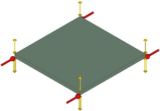
Let us consider now a problem of calculation of the steady-state temperature field for an infinite flat plate that radiates to the external environment. On the edges of the plate (along the length), we maintain the constant temperature of T=500 oK (we assume that for this temperature the effect of radiation for this plate will be significant). Radiation will take place from the surface of the plate at both sides of the plate to the external environment with the temperature equal to Text=293 oK. Now assuming the steady-state, we determine the temperature field on the surface of the plate at control points that are designated by the sensors (located along the OХ-axis).

Characteristics of the plate: thickness d=5 mm; width l=100 mm; thermal conductivity K=50 W/(m • oK); emissivity α=1. We maintain the zero heat flux along the boundary of a width of the plate. (see figure).

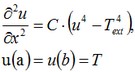
Let us consider the differential equation for this problem. Since the thermal heat flux on the opposite edges of the plate is equal to zero, the temperature field will be changing only along the length of the plate. By selecting the coordinate system such that the OX-axis is directed along the width of the plate and the OY-axis along the length, we will obtain the solution that depends only on the width of the plate. We will place the origin of the coordinate system О at the center of the plate. The equation will then take the form:

where the constant С is determined by taking into account the width of the plate as:

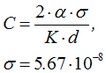
where σ – Boltzmann constant.

The analytical solution for this problem can be found as a Taylor’s series expansion. It can also be obtained numerically in the system Maple 9.5. We will consider the value along the length only up to the middle point, i.e., the selected origin of the coordinate system, since the solution is an even function (from the physical point of view it is obvious because we have equal temperature along the edges and the material is isotropic. In the center we will have the point of minimum since the body looses heat).

Let us represent now the analytical solution for the problem as a series. We note that

since from the physical point of view the plate could not cool down to the temperature below the temperature of the ambient environment. Hence, ∂u/∂x grows in a monotonous manner from -  to +  and that means that it has a single point of intersection with the OX-axis which will be the point of minimum of the solution. In the neighborhood of this point we expand the solution in a series:

By differentiating the given equation, we will obtain the expressions for the higher-order derivatives:

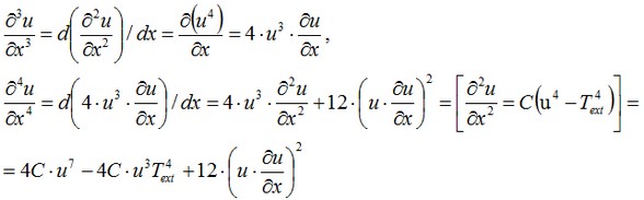
and so on. It is obvious that all derivatives can be represented in the form of a polynomial F of function u and the values of its first derivative

For all odd derivatives, all the terms of the polynomial F will contain as a factor the first derivative and therefore at the point of extremum we have

Hence the solution will take the form:

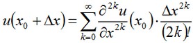
It is obvious from the symmetry of boundary conditions that the point x0 coincides with the selected zero O of the coordinate system.

There is no simple analytical solution for since on each step of calculation of the sum of the series,  we need to store all the coefficients of the polynomial F to evaluate the derivative for the next step. That is why we used standard ways of analytical evaluation of the derivative via the system Maple 9.52*.

The value of u at a point x0 was obtained in the following way: we select partial sums of the Taylor’s series at a point x0 +l/2 and equate them to the boundary value of the temperature T. Solution of these equations can be found numerically and, moreover, only the real positive roots were of interest. As a result we obtained u(0) = 467.4671303.

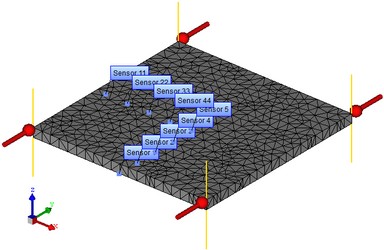
Let us locate the sensors of the temperature as shown on the Figure and make a plot for them at Y =0; 12.5; 25; 37.5 mm. In the given points we will compare the numerical solution obtained using AutoFEM Analysis with the analytical solution.

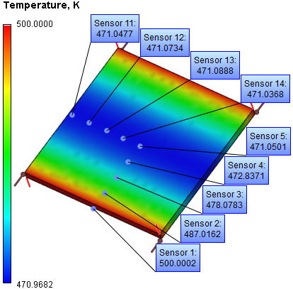
After carrying out calculation the following results are obtained:

Table 1. Parameters of finite element mesh

Table 2. Result "Temperature"

 

Conclusions:

The relative error of the numerical solution compared to the analytical solution is equal to 0.8% (on the axis of the plate). Notice that when the mesh is refined, convergence of the numerical solution to the analytical solution is slower for problems with radiation since the problem is nonlinear.

When solving a nonlinear problem it does not matter which elements are used for calculation: linear or quadratic.

*The results of numerical tests depend on the finite element mesh and may differ slightly from those given in the table.

**   In the cycle over the number of the terms in the series  we performed differentiation  and substitution of the fourth power of the solution instead of second derivative  and of zero instead of the first derivative into the final expression.

 

Read more about AutoFEM Thermal Analysis

autofem.com

Return to contents