Temperature Field of a Thermal System of a Heat Sink and a Chip

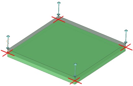
Let us consider a system consisting of a heat sink and a chip. The heat sink has a thermal conductivity equal to Khs=390 W/(m•oK), and a chip has a conductivity equal to Kchip=50 W/(m • oK) [Copper & Alloy Steel (SS)]. The chip is a source of heat which has a power of P=65 W. Along the entire interface between the heat sink and the chip there is a thermal contact with the thermal resistance equal to R=2•10-4 m2 • oK / W. The heat sink diffuses the heat with the heat transfer coefficient equal to h=3000 W/(m2 • oС) to the ambient environment that has a temperature of T0=293.15 oK. It is required to find the steady-state temperature distribution in the heat sink and in the microcircuit. We assume the worst case scenario: the heat is dissipated only by the  heat sink, i.e., all other heat losses are ignored. The thickness of the heat sink is b-a=1.5 mm. The thickness of the chip is a=1.5 mm. Both elements have rectangular shape with the volumes equal to Vhs=(b-a)•S and Vchip = a•S respectively, where S=30x30 mm=900•10-6 m2 – area of the interface. (see figure).

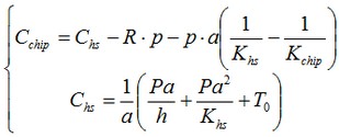
Let us consider now the change in the field across the thickness of the system. Let z be the height measured from the foundation of the chip. Then the differential equation takes the form:

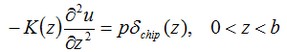
where δchip – function of a heat source – microcircuit. In our case, this heat source – is a segment of length a.

p – power distributed on this segment. If in the volume Vchip we apply the power P, then on the segment [0, a] p=P/Vchip.

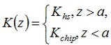
K(z) – is a function of thermal conductivity that can be defined in the following way:

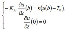
For this equation, the boundary conditions have the form:

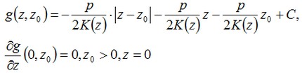
For a point source of the heat, the solution of a problem with homogeneous boundary condition will take the form:

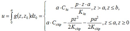
Solution u for a heat source has the form:

Constants Сhs and Cchip are determined from the following conditions:

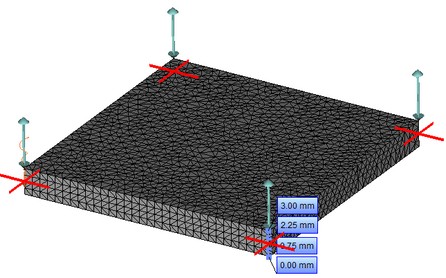
Let us locate the sensors of the temperature along the thickness; in 3D model they are located along the thickness of the plate. In the given points we will compare the numerical solution obtained using AutoFEM Analysis with the analytical solution.

Let us compare analytical solution with the solution obtained from AutoFEM. After carrying out calculation the following results are obtained:

Table 1. Parameters of finite element mesh

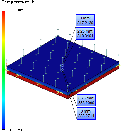
Table 2. Result "Temperature"

 

 

In addition, let us check the magnitude of the heat flux on the interface between the materials of the chip and heat sink, and also on the upper boundary that diffuses the heat. The important fact for us is that the heat flux, unlike the temperature, is a continuous function. The expression for the heat flux is given below:

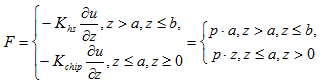
We can see from the analytical expression for the heat flux that inside the body of a heat sink (to which the heat power is applied) the heat flux is equal to a constant value. On the boundary pa = pz for z=a, and hence the continuity of the heat flux is satisfied.

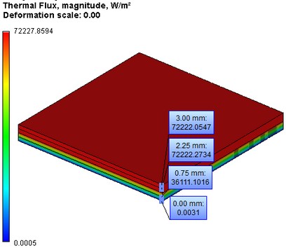
Table 3. Result "Thermal flux, W/m2"

Conclusions:

The relative error of the numerical solution compared with the analytical solution not exceed 0.34% for linear elements.

This problem was solved very accurately because solution was a piecewise continuous function with linear and quadratic parts.

The solution itself constitutes a quadratic function of temperature, and hence can be represented exactly using quadratic elements.

*The results of numerical tests depend on the finite element mesh and may differ slightly from those given in the table.

 

 

Read more about AutoFEM Thermal Analysis

autofem.com

 

Return to contents